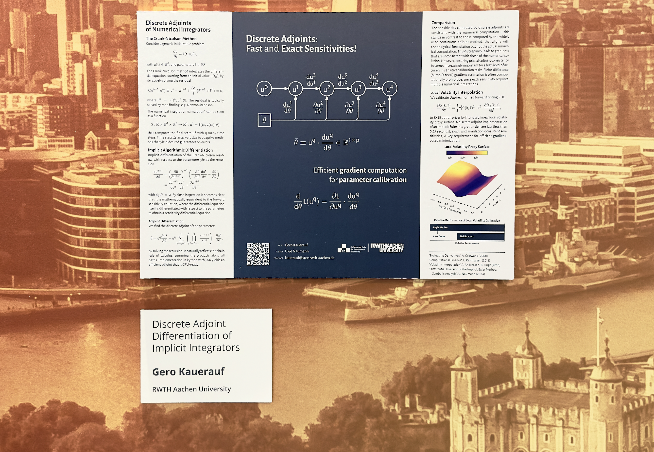
Check out my Poster (PDF) !

Discrete Adjoint Differentiation

Formally, vector adjoint algorithmic differentiation of a function \(F\colon\R^n\to\R^m,\,y=F(x)\) yields an vectorized adjoint model

where the vector-jacobian product (VJP) \[ \bar{X} = \bar{Y}\cdot F’(x), \] is computed by seeding the adjoint of the output \(\bar{Y}\in\R^{m\times m}\) and harvested from the adjoint of the input \(\bar{X}\in\R^{m\times n}\). The VJP is typically computed by propagating the seed matrix backwards through the computational graph \(G=(V,E)\) according to the chain rule of calculus

where \(P_{ij} = P(x_i, y_j)\) denotes the set of all paths from \(v_i = x_i\) to \(v_{n+\ell+j} = y_j\).

For the common case of scalar valued loss function \[ L\colon\R^n\to\R,\, y = L(\theta) , \] and the computation of its gradient, adjoint mode boils down to just \[ \bar{\theta} = \bar{y}\cdot \dv{L}{\theta} , \] where \(\bar{\theta} = \left(\nabla L\right)^T\) when seeding \(\bar{y} = 1\). This means that we can compute the gradient at the cost of a single function evaluation¹.

Implicit Differentiation

Consider a residual function \(R\colon\R^n\times\R^n\to\R^n\) that is used for the calibration of parameters \(\theta\) of some nonlinear, iterative model \(F\colon\R^n\to\R^n,\, y=F(\theta)\). Thus, we can express the residual as \(R(F(\theta), \theta)\). Assume that \(R\) vanishes identically at some solution \(\theta\), i.e.

that is computed by an beast of an iterative solver that barely any human understands. In the context of parameter calibration we are interested in the derivative of \(F\) with respect to \(\theta\). Naively, this would require differentiation through this monstrosity of a solver which is highly unstable and most often also very painful for the programmer (victim). To not have to do this, we first compute a solution (using the solver) and then differentiate the residual at the solution which yields

Reformulation for the derivative of interest gives us

Hence, we can compute the derivative of the model with respect to its parameters without the need of differentiating through the solution process at all. Most sophisticated AD tools (allow the user to) make use of this technique.

Discrete Adjoints of Differential Equations

Many initial value problems

with \(u(t)\in\R^n\), and parameters \(\theta\in\R^p\), are solved by implicit time integration schemes such as the Crank-Nicolson method that iteratively solves the residual

to compute a final state \(u^q\).

On the Poster (PDF) you can see how we differentiate through the whole intergration process by implicity differentiating every time step. This allows for an efficient computation of parameter sensitivies which we illustrate by directly calibrating Dupire’s PDE to market data by fitting a local volatility proxy surface.

[Todo: References]